.ipynb .pdf

repository open issue

Binder

Contents

Data

Note

If you’re in COLAB or have a local CUDA GPU, you can follow along with the more computationally intensive training in this lesson.

For those in COLAB, ensure the session is using a GPU by going to: Runtime > Change runtime type > Hardware accelerator = GPU.

# if you're using colab, then install the required modules
import sys

IN_COLAB = "google.colab" in sys.modules
if IN_COLAB:
    %pip install --quiet --upgrade pytorch-lightning lightning-bolts

Tensors

NumPy

import numpy as np

np.random.normal(size=(1,))  # scalar

array([0.80461192])

np.random.normal(size=(3,))  # vector

array([-0.60601988, -1.1925807 , -0.85305955])

np.random.normal(size=(3, 3))  # matrix

array([[ 0.38152432,  0.62216473,  1.62499855],
       [ 0.19659617,  1.4837946 ,  2.2099155 ],
       [-0.79474516,  0.15420569,  1.22662056]])

TensorFlow

Tensors are immutable.

There are also sparse tensors (mostly zeros), and a range of other data structures such as variables.

You can do a range mathematics with tensors.

import tensorflow as tf

2022-05-05 15:43:50.297814: W tensorflow/stream_executor/platform/default/dso_loader.cc:64] Could not load dynamic library 'libcudart.so.11.0'; dlerror: libcudart.so.11.0: cannot open shared object file: No such file or directory
2022-05-05 15:43:50.297847: I tensorflow/stream_executor/cuda/cudart_stub.cc:29] Ignore above cudart dlerror if you do not have a GPU set up on your machine.

tf.random.normal(shape=(1,))  # scalar

2022-05-05 15:43:51.825851: W tensorflow/stream_executor/platform/default/dso_loader.cc:64] Could not load dynamic library 'libcuda.so.1'; dlerror: libcuda.so.1: cannot open shared object file: No such file or directory
2022-05-05 15:43:51.825882: W tensorflow/stream_executor/cuda/cuda_driver.cc:269] failed call to cuInit: UNKNOWN ERROR (303)
2022-05-05 15:43:51.825905: I tensorflow/stream_executor/cuda/cuda_diagnostics.cc:156] kernel driver does not appear to be running on this host (fv-az90-458): /proc/driver/nvidia/version does not exist
2022-05-05 15:43:51.826237: I tensorflow/core/platform/cpu_feature_guard.cc:151] This TensorFlow binary is optimized with oneAPI Deep Neural Network Library (oneDNN) to use the following CPU instructions in performance-critical operations:  AVX2 AVX512F FMA
To enable them in other operations, rebuild TensorFlow with the appropriate compiler flags.

<tf.Tensor: shape=(1,), dtype=float32, numpy=array([-0.24286436], dtype=float32)>

tf.random.normal(shape=(3,))  # vector

<tf.Tensor: shape=(3,), dtype=float32, numpy=array([1.6570237, 0.2973419, 0.483523 ], dtype=float32)>

tf.random.normal(shape=(3, 3))  # matrix

<tf.Tensor: shape=(3, 3), dtype=float32, numpy=
array([[-0.15089877,  0.717702  , -0.10306445],
       [ 0.5718113 ,  0.42772955,  0.0218529 ],
       [ 1.3694383 ,  0.70673513,  0.18487518]], dtype=float32)>

PyTorch

More information for doing maths with PyTorch tensors.

import torch

torch.rand(size=(1,))  # scalar

tensor([0.2556])

torch.rand(size=(3,))  # vector

tensor([0.5138, 0.8876, 0.0671])

torch.rand(size=(3, 3))  # matrix

tensor([[0.1650, 0.4104, 0.1762],
        [0.6532, 0.0703, 0.5126],
        [0.6474, 0.9302, 0.8726]])

Reproducibility

Use random seeds to assist reproducibility.

Python

import random

random.seed(42)

NumPy

Used by scikit-learn.

np.random.seed(42)

So, after running the random seed cell above (with 42), this next scalar should always return:

>>> np.random.normal(size=(1,))
array([0.49671415])

np.random.normal(size=(1,))

array([0.49671415])

scikit-learn

Any object that uses the random_state keyword, set it to rng (for random number generator) rather than None.

For example, random_state is used in:

• sklearn.model_selection.train_test_split

• sklearn.datasets.make_classification

• sklearn.model_selection.KFold

• sklearn.ensemble.RandomForestClassifier

rng = np.random.RandomState(42)
X_train, X_test, y_train, y_test = train_test_split(X, y, random_state=rng)

TensorFlow (Keras)

tf.keras.utils.set_random_seed(42)

PyTorch (Lightning)

For PyTorch, there are separate seeds for the CPU and GPU:

def set_seed(seed):
    # cpu
    random.seed(seed)  # python
    np.random.seed(seed)  # numpy
    torch.manual_seed(seed)  # torch

    # gpu
    if torch.cuda.is_available():
        torch.cuda.manual_seed(seed)
        torch.cuda.manual_seed_all(seed)

set_seed(42)

PyTorch Lightning also has its own seed function:

from pytorch_lightning import seed_everything

seed_everything(42)

Global seed set to 42

42

Additionaly, some operations on GPUs are implemented stochastically for efficiency. Check the documentation for details.

To make your GPU workflow deterministic, you may also need to set:

# in pytorch
torch.backends.cudnn.deterministic = True
torch.backends.cudnn.benchmark = False

# in pytorch lightning trainer
Trainer(deterministic=True)

# in the pytorch lightning dataloader
def seed_worker(worker_id):
    worker_seed = torch.initial_seed() % 2**32
    numpy.random.seed(worker_seed)
    random.seed(worker_seed)

generator = torch.Generator()
generator.manual_seed(42)

DataLoader(
    train_dataset,
    worker_init_fn=seed_worker,
    generator=generator,
)

Tip

It’s good practice to try and reproduce your own work, to check that this is working correctly.

Data pipelines

Data pipelines are good practice for your workflow for many reasons such as convenience, reproduciblity, and avoiding data leakage.

They are especially useful:

• When the data does not fit in memory.

• When the data requires pre-processing.

• To efficiently use hardware.

The steps can include:

• Extract e.g., read data from memory / storage.

• Transform e.g., pre-processing, batching, shuffling.

• Load e.g., transfer to GPU.

Data loading

scikit-learn

Datasets

sklearn.datasets has a range of toy and real-world datasets.

from sklearn import datasets

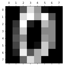
digits = datasets.load_digits()

import matplotlib.pyplot as plt

plt.gray()
plt.matshow(digits.images[0])
plt.show()

<Figure size 432x288 with 0 Axes>

df_california_housing = datasets.fetch_california_housing(as_frame=True)

df_california_housing["frame"]

	MedInc	HouseAge	AveRooms	AveBedrms	Population	AveOccup	Latitude	Longitude	MedHouseVal
0	8.3252	41.0	6.984127	1.023810	322.0	2.555556	37.88	-122.23	4.526
1	8.3014	21.0	6.238137	0.971880	2401.0	2.109842	37.86	-122.22	3.585
2	7.2574	52.0	8.288136	1.073446	496.0	2.802260	37.85	-122.24	3.521
3	5.6431	52.0	5.817352	1.073059	558.0	2.547945	37.85	-122.25	3.413
4	3.8462	52.0	6.281853	1.081081	565.0	2.181467	37.85	-122.25	3.422
...	...	...	...	...	...	...	...	...	...
20635	1.5603	25.0	5.045455	1.133333	845.0	2.560606	39.48	-121.09	0.781
20636	2.5568	18.0	6.114035	1.315789	356.0	3.122807	39.49	-121.21	0.771
20637	1.7000	17.0	5.205543	1.120092	1007.0	2.325635	39.43	-121.22	0.923
20638	1.8672	18.0	5.329513	1.171920	741.0	2.123209	39.43	-121.32	0.847
20639	2.3886	16.0	5.254717	1.162264	1387.0	2.616981	39.37	-121.24	0.894

20640 rows × 9 columns

Pipelines

You can create data pipelines via a list of key-value pairs:

from sklearn.pipeline import Pipeline

from sklearn.decomposition import PCA
from sklearn.svm import SVC

estimators = [("reduce_dim", PCA()), ("clf", SVC())]

Pipeline(estimators)

Pipeline(steps=[('reduce_dim', PCA()), ('clf', SVC())])

Or, by using the make_pipeline function and passing in instantiated classes:

from sklearn.pipeline import make_pipeline

from sklearn.naive_bayes import MultinomialNB
from sklearn.preprocessing import Binarizer

make_pipeline(Binarizer(), MultinomialNB())

Pipeline(steps=[('binarizer', Binarizer()), ('multinomialnb', MultinomialNB())])

TensorFlow (Keras)

Keras models accept three types of inputs:

• NumPy arrays

  • Suitable for when the data fits in memory.

• TensorFlow Dataset objects

  • Suitable for datasets that do not fit in memory and that are streamed from disk or from a distributed filesystem.

• Python generators

  • Suitable for custom processing that yields batches of data (subclasses of tf.keras.utils.Sequence class).

The documentation has more information on different data formats, such as CSV and Pandas DataFrames.

Note

The word class has two definitions here depending on the context.

• A class in Python bundles data and functionality together to make new object instances.

• The class in machine learning is the category that a sample belongs to e.g., cat or dog.

Keras features a range of utilities to help you turn raw data on disk into a Dataset:

• tf.keras.utils.image_dataset_from_directory turns image files sorted into class-specific folders into a labeled dataset of image tensors.

• tf.keras.utils.text_dataset_from_directory does the same for text files.

• tf.keras.utils.timeseries_dataset_from_array creates a dataset of sliding windows over a timeseries provided as array.

Tip

If you have a large dataset and you are training on GPU(s), consider using Dataset objects, since they will take care of performance-critical details, such as:

• Asynchronously preprocessing your data on CPU while your GPU is busy, and buffering it into a queue.

• Prefetching data on GPU memory so it’s immediately available when the GPU has finished processing the previous batch, so you can reach full GPU utilization.

Keras Utilities

import pathlib

import matplotlib.pyplot as plt

if IN_COLAB:
    dataset_url = "https://storage.googleapis.com/download.tensorflow.org/example_images/flower_photos.tgz"
    data_dir = tf.keras.utils.get_file(
        origin=dataset_url, fname="flower_photos", untar=True
    )
    data_dir = pathlib.Path(data_dir)

    BATCH_SIZE = 32
    IMAGE_HEIGHT = 180
    IMAGE_WIDTH = 180

    ds_train = tf.keras.utils.image_dataset_from_directory(
        data_dir,
        validation_split=0.2,
        subset="training",
        seed=123,
        image_size=(IMAGE_HEIGHT, IMAGE_WIDTH),
        batch_size=BATCH_SIZE,
    )

if IN_COLAB:
    class_names = ds_train.class_names

    plt.figure(figsize=(10, 10))
    for images, labels in ds_train.take(1):
        for i in range(9):
            ax = plt.subplot(3, 3, i + 1)
            plt.imshow(images[i].numpy().astype("uint8"))
            plt.title(class_names[labels[i]])
            plt.axis("off")

TensorFlow Datasets

Can split the data on load.

import tensorflow_datasets as tfds

if IN_COLAB:
    (ds_train, ds_val, ds_test), ds_info = tfds.load(
        "tf_flowers",
        split=["train[:80%]", "train[80%:90%]", "train[90%:]"],
        with_info=True,  # returns (img, label) instead of {image': img, 'label': label}
        as_supervised=True,
    )

NumPy to TensorFlow Dataset

Load a .npz file:

DATA_URL = "https://storage.googleapis.com/tensorflow/tf-keras-datasets/mnist.npz"

path = tf.keras.utils.get_file("mnist.npz", DATA_URL)
with np.load(path) as data:
    x_train = data["x_train"]
    y_train = data["y_train"]
    x_test = data["x_test"]
    y_test = data["y_test"]

type(x_train)

numpy.ndarray

Convert to a TensorFlow object:

ds_train = tf.data.Dataset.from_tensor_slices((x_train, y_train))
ds_test = tf.data.Dataset.from_tensor_slices((x_test, y_test))

ds_train

<TensorSliceDataset element_spec=(TensorSpec(shape=(28, 28), dtype=tf.uint8, name=None), TensorSpec(shape=(), dtype=tf.uint8, name=None))>

PyTorch (Lightning)

There are few different options for data:

• Dataset

  • Maps keys to data samples.

  • Also, Iterable Datasets for sequential data.

• DataLoader

  • Wraps an iterable around Dataset.

• LightningDataModule

  • A collection of training/validation/test/predict DataLoaders, along with their preprocessing/downloading steps.

Dataset

from torch.utils.data import random_split
from torchvision.datasets import MNIST

import os

data_path = f"{os.getcwd()}/data"

train_dataset = MNIST(data_path, train=True, download=True)
test_dataset = MNIST(data_path, train=False, download=True)
predict_dataset = MNIST(
    data_path, train=False, download=True
)  # same as the test dataset

train_dataset, val_dataset = random_split(train_dataset, [55000, 5000])

train_dataset

<torch.utils.data.dataset.Subset at 0x7eff89e53f70>

DataLoader

from torch.utils.data import DataLoader

BATCH_SIZE = 32

train_dataloader = DataLoader(train_dataset, batch_size=BATCH_SIZE)
val_dataloader = DataLoader(val_dataset, batch_size=BATCH_SIZE)
test_dataloader = DataLoader(test_dataset, batch_size=BATCH_SIZE)
predict_dataloader = DataLoader(predict_dataset, batch_size=BATCH_SIZE)

train_dataloader

<torch.utils.data.dataloader.DataLoader at 0x7eff89013b50>

LightningDataModule

Decouples the data hooks from the PyTorch Lightning model, so you can develop dataset agnostic models with reusable and sharable DataModules.

You can think of this as the data pipeline.

For multi-node training, you can also add prepare_data_per_node.

import pytorch_lightning as pl
from torchvision import transforms

class MNISTDataModule(pl.LightningDataModule):
    def __init__(self, data_path=data_path, batch_size=BATCH_SIZE):
        super().__init__()
        self.data_path = data_path
        self.batch_size = batch_size
        self.transform = transforms.Compose(
            [
                transforms.ToTensor(),
                transforms.Normalize((0.1307,), (0.3081,)),  # specific to MNIST
            ]
        )

    def prepare_data(self):
        # download data once, useful for distributed training to avoid duplicates
        MNIST(self.data_path, train=True, download=True)
        MNIST(self.data_path, train=False, download=True)

    def setup(self, stage=None):
        if stage == "fit" or stage is None:
            mnist_full = MNIST(self.data_path, train=True, transform=self.transform)
            self.mnist_train, self.mnist_val = random_split(mnist_full, [55000, 5000])

        if stage == "test" or stage is None:
            self.mnist_test = MNIST(
                self.data_path, train=False, transform=self.transform
            )

        if stage == "predict" or stage is None:
            self.mnist_predict = MNIST(
                self.data_path, train=False, transform=self.transform
            )

    def train_dataloader(self):
        return DataLoader(self.mnist_train, batch_size=self.batch_size)

    def val_dataloader(self):
        return DataLoader(self.mnist_val, batch_size=self.batch_size)

    def test_dataloader(self):
        return DataLoader(self.mnist_test, batch_size=self.batch_size)

    def predict_dataloader(self):
        return DataLoader(self.mnist_predict, batch_size=self.batch_size)

datamodule = MNISTDataModule()

You can then use the LightningDataModule in the Trainer:

trainer.fit(model, datamodule=datamodule)
trainer.test(datamodule=datamodule)

Now you can also swap out the datamodule for another one that works with the same model e.g., Fashion MNIST:

datamodule = FashionMNISTDataModule()

Shuffle

Shuffle the training data to help with training accuracy.

Normally, the test data is not shuffled.

TensorFlow (Keras)

ds_train = ds_train.shuffle(10_000)

ds_train

<ShuffleDataset element_spec=(TensorSpec(shape=(28, 28), dtype=tf.uint8, name=None), TensorSpec(shape=(), dtype=tf.uint8, name=None))>

PyTorch (Lightning)

BATCH_SIZE = 32

train_dataloader = DataLoader(train_dataset, shuffle=True)

train_dataloader

<torch.utils.data.dataloader.DataLoader at 0x7eff80570460>

Batch

A batch is a set of examples used in one iteration of model training.

The batch size is the number of examples in a batch.

The optimum batch size depends on the problem and what you’re optimising for.

In general:

• They are often multiples of 32, where 32 or 64 is a good starting point if unsure.

• Larger batch sizes can be more performant (e.g., 256 is often used for distributed training over multiple GPUs).

• Batch sizes that match the number of classes for multi-class classification can increase accuracy (e.g., 10 for MNIST).

TensorFlow (Keras)

BATCH_SIZE = 32

ds_train = ds_train.batch(batch_size=BATCH_SIZE)

ds_train

<BatchDataset element_spec=(TensorSpec(shape=(None, 28, 28), dtype=tf.uint8, name=None), TensorSpec(shape=(None,), dtype=tf.uint8, name=None))>

PyTorch (Lightning)

BATCH_SIZE = 32

train_dataloader = DataLoader(train_dataset, batch_size=BATCH_SIZE)

train_dataloader

<torch.utils.data.dataloader.DataLoader at 0x7eff805701c0>

Automatic batch size with PyTorch lightning:

Trainer(auto_scale_batch_size=True)

Map

Map a preprocessing function to a dataset.

TensorFlow (Keras)

dataset.map(function)

Tip

There are range of ways to improve the performance of the data pipeline.

In these examples, using tf.data.AUTOTUNE leaves the decision to TensorFlow.

Dataset caching

Cache the data after the first iteration through it. The data can be cached to either memory or a local file.

This can improve performance when:

• The data stays the same each iteration.

• The data is read from a remote distributed filesystem.

• The data is I/O (input/output) bound and fits in memory.

Note, large datasets are sharded rather than cached, as they don’t fit into memory.

TensorFlow (Keras)

ds_train = ds_train.cache()

ds_train

<CacheDataset element_spec=(TensorSpec(shape=(None, 28, 28), dtype=tf.uint8, name=None), TensorSpec(shape=(None,), dtype=tf.uint8, name=None))>

Prefetch data

Overlaps data pre-processing and model execution while training.

TensorFlow (Keras)

ds_train = ds_train.prefetch(buffer_size=tf.data.AUTOTUNE)

ds_train

<PrefetchDataset element_spec=(TensorSpec(shape=(None, 28, 28), dtype=tf.uint8, name=None), TensorSpec(shape=(None,), dtype=tf.uint8, name=None))>

Parallel data extraction

Extract the data in parallel.

TensorFlow (Keras)

dataset.interleave(
    build_dataset, 
    num_parallel_calls=tf.data.AUTOTUNE
)

PyTorch (Lightning)

Set num_workers to be greater than 0 in the DataLoader:

train_dataloader = DataLoader(train_dataset, num_workers=4)

Tip

Can also pin memory to the GPU for faster memory copies by adding pin_memory=True inside the DataLoader.

Data pre-processing

Pre-processing your data is often helpful as the raw data is often not in the exact format that the model performs well with.

For example, normalising the values in a tensor can help with model training.

Tip

Pre-processing transformations are based on the training data only (not the test data). For example, if you normalise by the avergage, ensure that this is the average of the training data only.

These are then applied to the inputs of both the training and the test data.

This helps avoid data leakage of the test data into training.

scikit-learn

from sklearn import preprocessing

preprocessing.StandardScaler()  # standardisation: zero mean and unit variance

StandardScaler()

preprocessing.Normalizer()  # normalisation: unit norm

Normalizer()

preprocessing.PowerTransformer()  # mapping to Gaussian distribution

PowerTransformer()

preprocessing.OneHotEncoder()  # encoding categorical features

OneHotEncoder()

TensorFlow (Keras)

tf.keras.layers.Rescaling(1.0 / 255)

<keras.layers.preprocessing.image_preprocessing.Rescaling at 0x7eff8901f580>

PyTorch (Lightning)

import torchvision

torchvision.transforms.Normalize((0.1307,), (0.3081,)),  # specific to MNIST

(Normalize(mean=(0.1307,), std=(0.3081,)),)

Data augmentation

Data augmentation artificially increases the range and number of training examples.

This is useful for small data sets.

There are a range of methods. For example, in image problems you could rotate, stretch, and reflect images.

Tip

Apply random transformations after both caching (to avoid caching randomness) and batching (for vectorisation).

TensorFlow (Keras)

tf.keras.layers.RandomFlip("horizontal")

<keras.layers.preprocessing.image_preprocessing.RandomFlip at 0x7eff80539430>

tf.keras.layers.RandomRotation(0.1)

<keras.layers.preprocessing.image_preprocessing.RandomRotation at 0x7eff805395b0>

PyTorch (Lightning)

torchvision.transforms.RandomHorizontalFlip()

RandomHorizontalFlip(p=0.5)

torchvision.transforms.RandomRotation(0.1)

RandomRotation(degrees=[-0.1, 0.1], interpolation=nearest, expand=False, fill=0)

Parallel data transformation

Pre-process your data in parallel.

TensorFlow (Keras)

dataset.map(
    function, 
    num_parallel_calls=tf.data.AUTOTUNE
)

Vectorise mapping

Batch before mapping, to vectorise a function.

TensorFlow (Keras)

dataset.batch(256).map(function)

Mixed precision

Mixed precision is the combined use of 16-bit and 32-bit floating-point types during training to use less memory and make it run faster.

It uses 32-bits where it needs to for accuracy and 16-bits elsewhere for speed.

Note

This functionality varies by GPU, and is mostly available to modern NVIDIA GPUs.

Warning

Be careful with underflow and overflow issues.

16-bit floats above 65,504 overflow to infinity and below 6.0_x10^-8 underflow to zero.

Loss scaling can help avoid errors by scaling the losses up or down temporarily i.e.,:
optimizer = mixed_precision.LossScaleOptimizer(optimizer)

TensorFlow (Keras)

tf.keras.mixed_precision.set_global_policy('mixed_float16')

PyTorch (Lightning)

Trainer(precision=16)

Example - Digit Classification

TensorFlow Datasets

TensorFlow Datasets is a collection of datasets ready to use, with TensorFlow or other Python ML frameworks.

Here is an example for MNIST.

Load the data:

(ds_train, ds_val, ds_test), ds_info = tfds.load(
    "mnist",
    split=["train[:80%]", "train[80%:90%]", "train[90%:]"],
    shuffle_files=True,  # good practise for larger datasets with many files on disk
    as_supervised=True,
    with_info=True,
)

2022-05-05 15:43:56.256555: W tensorflow/core/platform/cloud/google_auth_provider.cc:184] All attempts to get a Google authentication bearer token failed, returning an empty token. Retrieving token from files failed with "NOT_FOUND: Could not locate the credentials file.". Retrieving token from GCE failed with "FAILED_PRECONDITION: Error executing an HTTP request: libcurl code 6 meaning 'Couldn't resolve host name', error details: Could not resolve host: metadata".

Downloading and preparing dataset 11.06 MiB (download: 11.06 MiB, generated: 21.00 MiB, total: 32.06 MiB) to /home/runner/tensorflow_datasets/mnist/3.0.1...

Dataset mnist downloaded and prepared to /home/runner/tensorflow_datasets/mnist/3.0.1. Subsequent calls will reuse this data.

Create the data pipelines:

AUTOTUNE = tf.data.AUTOTUNE


def normalise_image(image, label):
    return tf.cast(image, tf.float32) / 255.0, label


def training_pipeline(ds_train):
    ds_train = ds_train.map(
        normalise_image, num_parallel_calls=AUTOTUNE
    )  # parallelise preprocessing first to reuse it
    ds_train = ds_train.cache()  # cache before shuffling for performance
    ds_train = ds_train.shuffle(
        ds_info.splits["train"].num_examples
    )  # shuffle by the full dataset size
    ds_train = ds_train.batch(
        128
    )  # batch after shuffling for unique batches at each epoch
    ds_train = ds_train.prefetch(
        AUTOTUNE
    )  # end pipeline with prefetching for performance
    return ds_train


def test_pipeline(ds_test):
    ds_test = ds_test.map(normalise_image, num_parallel_calls=AUTOTUNE)
    ds_test = ds_test.batch(128)
    ds_test = ds_test.cache()
    # cache after batching because batches can be the same between epochs
    # no shuffling needed
    ds_test = ds_test.prefetch(AUTOTUNE)
    return ds_test


ds_train = training_pipeline(ds_train)
ds_val = training_pipeline(ds_val)
ds_test = test_pipeline(ds_test)

Create the model using the Functional API:

inputs = tf.keras.Input(shape=(28, 28, 1), name="inputs")
x = tf.keras.layers.Flatten(name="flatten")(inputs)
x = tf.keras.layers.Dense(128, activation="relu", name="layer1")(x)
x = tf.keras.layers.Dense(128, activation="relu", name="layer2")(x)
outputs = tf.keras.layers.Dense(10, name="outputs")(x)

model = tf.keras.Model(inputs, outputs, name="functional")

model.summary()

Model: "functional"

_________________________________________________________________

 Layer (type)                Output Shape              Param #   

=================================================================

 inputs (InputLayer)         [(None, 28, 28, 1)]       0         

 flatten (Flatten)           (None, 784)               0         

 layer1 (Dense)              (None, 128)               100480    

 layer2 (Dense)              (None, 128)               16512     

 outputs (Dense)             (None, 10)                1290      

=================================================================

Total params: 118,282

Trainable params: 118,282

Non-trainable params: 0

_________________________________________________________________

Compile the model:

model.compile(
    optimizer=tf.keras.optimizers.Adam(),
    loss=tf.keras.losses.SparseCategoricalCrossentropy(from_logits=True),
    metrics=[tf.keras.metrics.SparseCategoricalAccuracy(name="accuracy")],
)

Train the model:

NUM_EPOCHS = 10

history = model.fit(
    ds_train,
    validation_data=ds_val,
    epochs=NUM_EPOCHS,
    verbose=False,
);

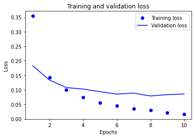
View the loss and accuracy curves over the epochs:

import matplotlib.pyplot as plt

epochs_range = range(1, NUM_EPOCHS + 1)

plt.plot(epochs_range, history.history["loss"], "bo", label="Training loss")
plt.plot(epochs_range, history.history["val_loss"], "b", label="Validation loss")
plt.title("Training and validation loss")
plt.xlabel("Epochs")
plt.ylabel("Loss")
plt.legend()
plt.show()

plt.plot(epochs_range, history.history["accuracy"], "bo", label="Training accuracy")
plt.plot(
    epochs_range, history.history["val_accuracy"], "b", label="Validation accuracy"
)
plt.title("Training and validation accuracy")
plt.xlabel("Epochs")
plt.ylabel("Accuracy")
plt.ylim([0.9, 1.0])
plt.legend()
plt.show()

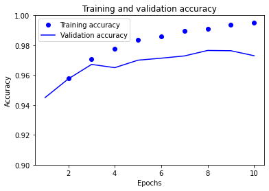
The training accuracy and the validation accuracy are diverging.

This means that the model is overfitting (i.e., memorising the training data and not generalising to the validation data).

One way to alleviate this is to add regularisation.

In this example, we’ll add dropout to the dense layers.

inputs = tf.keras.Input(shape=(28, 28, 1), name="inputs")
x = tf.keras.layers.Flatten(name="flatten")(inputs)
x = tf.keras.layers.Dense(128, activation="relu", name="layer1")(x)

# I'm new
x = tf.keras.layers.Dropout(0.2)(x)

x = tf.keras.layers.Dense(128, activation="relu", name="layer2")(x)
outputs = tf.keras.layers.Dense(10, name="outputs")(x)

model = tf.keras.Model(inputs, outputs, name="functional")

model.compile(
    optimizer=tf.keras.optimizers.Adam(),
    loss=tf.keras.losses.SparseCategoricalCrossentropy(from_logits=True),
    metrics=[tf.keras.metrics.SparseCategoricalAccuracy(name="accuracy")],
)

history = model.fit(
    ds_train,
    validation_data=ds_val,
    epochs=NUM_EPOCHS,
    verbose=False,
);

plt.plot(epochs_range, history.history["accuracy"], "bo", label="Training accuracy")
plt.plot(
    epochs_range, history.history["val_accuracy"], "b", label="Validation accuracy"
)
plt.title("Training and validation accuracy")
plt.xlabel("Epochs")
plt.ylabel("Accuracy")
plt.ylim([0.9, 1.0])
plt.legend()
plt.show()

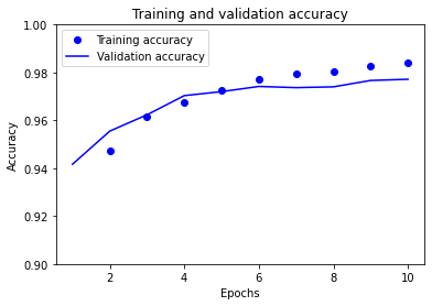
Much better. The model now performs well on both the training and validation data.

PyTorch (Lightning)

import os

import torch
import torch.nn.functional as F
from pytorch_lightning import (
    LightningDataModule,
    LightningModule,
    Trainer,
    seed_everything,
)
from pytorch_lightning.callbacks.progress import TQDMProgressBar
from torch import nn
from torch.utils.data import DataLoader, random_split
from torchmetrics.functional import accuracy
from torchvision import transforms
from torchvision.datasets import CIFAR10, MNIST

Set global parameters:

seed_everything(42)

Global seed set to 42

42

PATH_DATASETS = f"{os.getcwd()}/data"
AVAIL_GPUS = min(1, torch.cuda.device_count())
BATCH_SIZE = 256 if AVAIL_GPUS else 64

Create the (dataset agnostic) PyTorch Lightning Model:

class LitModel(LightningModule):
    def __init__(
        self, channels, width, height, num_classes, hidden_size=64, learning_rate=2e-4
    ):

        super().__init__()

        # We take in input dimensions as parameters and use those to dynamically build model.
        self.channels = channels
        self.width = width
        self.height = height
        self.num_classes = num_classes
        self.hidden_size = hidden_size
        self.learning_rate = learning_rate

        self.model = nn.Sequential(
            nn.Flatten(),
            nn.Linear(channels * width * height, hidden_size),
            nn.ReLU(),
            nn.Dropout(0.1),
            nn.Linear(hidden_size, hidden_size),
            nn.ReLU(),
            nn.Dropout(0.1),
            nn.Linear(hidden_size, num_classes),
        )

    def forward(self, x):
        x = self.model(x)
        return F.log_softmax(x, dim=1)

    def training_step(self, batch, batch_idx):
        x, y = batch
        logits = self(x)
        loss = F.nll_loss(logits, y)
        return loss

    def validation_step(self, batch, batch_idx):
        x, y = batch
        logits = self(x)
        loss = F.nll_loss(logits, y)
        preds = torch.argmax(logits, dim=1)
        acc = accuracy(preds, y)
        self.log("val_loss", loss, prog_bar=True)
        self.log("val_acc", acc, prog_bar=True)
        return loss

    def test_step(self, batch, batch_idx):
        # Here we just reuse the validation_step for testing
        return self.validation_step(batch, batch_idx)

    def configure_optimizers(self):
        optimizer = torch.optim.Adam(self.parameters(), lr=self.learning_rate)
        return optimizer

Create the PyTorch Lightning DataModule:

class MNISTDataModule(LightningDataModule):
    def __init__(self, data_dir=PATH_DATASETS):
        super().__init__()
        self.data_dir = data_dir
        self.transform = transforms.Compose(
            [
                transforms.ToTensor(),
                transforms.Normalize((0.1307,), (0.3081,)),  # specific to MNIST
            ]
        )

    def prepare_data(self):  # download the data, once if distributed
        MNIST(self.data_dir, train=True, download=True)
        MNIST(self.data_dir, train=False, download=True)

    def setup(self, stage=None):
        # Assign train/val datasets for use in dataloaders
        if stage == "fit" or stage is None:
            ds_full = MNIST(self.data_dir, train=True, transform=self.transform)
            self.ds_train, self.ds_val = random_split(ds_full, [55000, 5000])

        # Assign test dataset for use in dataloader(s)
        if stage == "test" or stage is None:
            self.ds_test = MNIST(self.data_dir, train=False, transform=self.transform)

    def train_dataloader(self):
        return DataLoader(self.ds_train, batch_size=BATCH_SIZE)

    def val_dataloader(self):
        return DataLoader(self.ds_val, batch_size=BATCH_SIZE)

    def test_dataloader(self):
        return DataLoader(self.ds_test, batch_size=BATCH_SIZE)

Instantiate the Model, DataModule, and Trainer:

datamodule = MNISTDataModule()

model = LitModel(channels=1, width=28, height=28, num_classes=10)

trainer = Trainer(
    gpus=AVAIL_GPUS,
    max_epochs=3,
    callbacks=TQDMProgressBar(refresh_rate=20),
)

GPU available: False, used: False

TPU available: False, using: 0 TPU cores

IPU available: False, using: 0 IPUs

HPU available: False, using: 0 HPUs

Run training:

if IN_COLAB:
    trainer.fit(model, datamodule=datamodule)

Test the model:

if IN_COLAB:
    trainer.test(datamodule=datamodule)

Now, we can change over to a different dataset e.g., CIFAR10:

class CIFAR10DataModule(LightningDataModule):
    def __init__(self, data_dir=PATH_DATASETS):
        super().__init__()
        self.data_dir = data_dir
        self.transform = transforms.Compose(
            [
                transforms.ToTensor(),
                transforms.Normalize(
                    (0.5, 0.5, 0.5), (0.5, 0.5, 0.5)
                ),  # specific to CIFAR10
            ]
        )

    def prepare_data(self):  # download the data, once if distributed
        CIFAR10(self.data_dir, train=True, download=True)
        CIFAR10(self.data_dir, train=False, download=True)

    def setup(self, stage=None):
        # Assign train/val datasets for use in dataloaders
        if stage == "fit" or stage is None:
            ds_full = CIFAR10(self.data_dir, train=True, transform=self.transform)
            self.ds_train, self.ds_val = random_split(ds_full, [45000, 5000])

        # Assign test dataset for use in dataloader(s)
        if stage == "test" or stage is None:
            self.ds_test = CIFAR10(self.data_dir, train=False, transform=self.transform)

    def train_dataloader(self):
        return DataLoader(self.ds_train, batch_size=BATCH_SIZE)

    def val_dataloader(self):
        return DataLoader(self.ds_val, batch_size=BATCH_SIZE)

    def test_dataloader(self):
        return DataLoader(self.ds_test, batch_size=BATCH_SIZE)

datamodule = CIFAR10DataModule()

model = LitModel(channels=3, width=32, height=32, num_classes=10, hidden_size=512)

trainer = Trainer(
    gpus=AVAIL_GPUS,
    max_epochs=3,
    callbacks=TQDMProgressBar(refresh_rate=20),
)

GPU available: False, used: False

TPU available: False, using: 0 TPU cores

IPU available: False, using: 0 IPUs

HPU available: False, using: 0 HPUs

if IN_COLAB:
    trainer.fit(model, datamodule=datamodule)

if IN_COLAB:
    trainer.test(datamodule=datamodule)

This simple model works well for MNIST but not for CIFAR10. However, it demonstrates the ease and benefits of switching out data modules.

PyTorch Lightning Bolts simplifies this even further for common DataModules (e.g., MNIST, FashionMNIST, CIFAR10, ImageNet) by providing them for you:

from pl_bolts.datamodules import MNISTDataModule

datamodule = MNISTDataModule(PATH_DATASETS)

model = LitModel(channels=1, width=28, height=28, num_classes=10)

trainer = Trainer(
    gpus=AVAIL_GPUS,
    max_epochs=3,
    callbacks=TQDMProgressBar(refresh_rate=20),
)

GPU available: False, used: False

TPU available: False, using: 0 TPU cores

IPU available: False, using: 0 IPUs

HPU available: False, using: 0 HPUs

if IN_COLAB:
    trainer.fit(model, datamodule=datamodule)

if IN_COLAB:
    trainer.test(datamodule=datamodule)

PyTorch Lighting Bolts also has a range of models (e.g., regression, GPT-2, ImageGPT, GAN, VAE):

from pl_bolts.models.vision import ImageGPT

Also, you can override functionality for fast iteration of research ideas:

class VideoGPT(ImageGPT):  # inherit from the pre-trained model
    def training_step(self, batch, batch_idx):  # create a new training step
        # cool science

Questions

Question 1

Should I split my data in train and test subsets before or after pre-processing?

Question 2

Before I use random functionality, what is a good practice for reproducibility?

Question 3

What should I create if there are multiple steps to my data pre-processing?

Question 4

Name three ways to improve performance in a data pipeline.

Solutions

Key Points

Important

• Always split the data into train and test subsets first, before any pre-processing.

• Never fit to the test data.

• Use a data pipeline.

• Use a random seed and any available deterministic functionalities for reproducibility.

  • Try and reproduce your own work, to check that it is reproducible.

• Consider optimising the data pipeline with:

  • Shuffling.

  • Batching.

  • Caching.

  • Prefetching.

  • Parallel data extraction.

  • Data augmentation.

  • Parallel data transformation.

  • Vectorised mapping.

  • Mixed precision.

Further information

Good practices

• Do data processing in a pipeline or module to increase portability and reproducibility.

• Pre-processing transformations are based on the training data only (not the test data). These are then applied to the inputs of both the training and the test data. This helps avoid data leakage.

• Analyse data pipeline performance with TensorBoard Profiler.

• Use sparse tensors when there are many zeros / np.nans (e.g., TensorFlow).

• Take care with datasets with imbalanced classes (i.e., only a few positive samples).

• Best practices for managing data with PyTorch Lightning and scikit-learn.

• Models are often heavily optimised, while the data is less so. There are many good practices around data-centric machine learning.

• Consider sharing your data for reproducibility if you can.

Other options

• NVIDIA Data Loading Library (DALI)

  • A library for data loading and pre-processing to accelerate deep learning applications.

• Ray Datasets

  • Load and exchange data in Ray libraries and applications.

• NVIDIA Replicator Composer

  • A tool for creating synthetic data.

Resources

• Papers with code - Datasets

• HuggingFace - Datasets

• Google research datasets

• Google Dataset Search

• Google Cloud public datasets

• Kaggle Datasets

• Torch Vision Datasets

• Torch Text Datasets

• Torch Audio Datasets

previous

Tools

next

Models