Summary and Setup
Welcome to SWD1a: Introduction to Python
This website contains materials from The Carpentries, with some small modifications to tailor it to our needs for SWD1a: Introduction to Python here at the University of Leeds.
Please refer to your course hackpad for additional links, topics, and discussion points specific to your course.
The format of this workshop
The best way to learn how to program is to do something useful, so this introduction to Python is built around a common scientific task: data analysis.
Scenario: A Miracle Arthritis Inflammation Cure
Our imaginary colleague “Dr. Maverick” has invented a new miracle drug that promises to cure arthritis inflammation flare-ups after only 3 weeks since initially taking the medication! Naturally, we wish to see the clinical trial data, and after months of asking for the data they have finally provided us with a CSV spreadsheet containing the clinical trial data.
The CSV file contains the number of inflammation flare-ups per day for the 60 patients in the initial clinical trial, with the trial lasting 40 days. Each row corresponds to a patient, and each column corresponds to a day in the trial. Once a patient has their first inflammation flare-up they take the medication and wait a few weeks for it to take effect and reduce flare-ups.
To see how effective the treatment is we would like to:
- Calculate the average inflammation per day across all patients.
- Plot the result to discuss and share with colleagues.
Data Format
The data sets are stored in comma-separated values (CSV) format:
- each row holds information for a single patient,
- columns represent successive days.
The first three rows of our first file look like this:
0,0,1,3,1,2,4,7,8,3,3,3,10,5,7,4,7,7,12,18,6,13,11,11,7,7,4,6,8,8,4,4,5,7,3,4,2,3,0,0
0,1,2,1,2,1,3,2,2,6,10,11,5,9,4,4,7,16,8,6,18,4,12,5,12,7,11,5,11,3,3,5,4,4,5,5,1,1,0,1
0,1,1,3,3,2,6,2,5,9,5,7,4,5,4,15,5,11,9,10,19,14,12,17,7,12,11,7,4,2,10,5,4,2,2,3,2,2,1,1
Each number represents the number of inflammation bouts that a particular patient experienced on a given day.
For example, value “6” at row 3 column 7 of the data set above means that the third patient was experiencing inflammation six times on the seventh day of the clinical study.
In order to analyze this data and report to our colleagues, we’ll have to learn a little bit about programming.
Prerequisites
You need to understand the concepts of files and directories and how to start a Python interpreter before tackling this lesson. This lesson sometimes references Jupyter Notebook although you can use any Python interpreter mentioned in the Setup.
The commands in this lesson pertain to any officially supported Python version, currently Python 3.8+. Newer versions usually have better error printouts, so using newer Python versions is recommend if possible.
Getting Started
To get started, follow the directions on the Setup page to open up Google colab. After the course, you can follow the intructions here to install a Python interpreter locally on your machine.
Overview
This lesson is designed to be run on a personal computer. All of the software and data used in this lesson are freely available online, and instructions on how to obtain them are provided below.
Get Python
In this lesson, we will be using Python 3 with some of its most popular scientific libraries. We are going to be using Google Colab, a hosted Jupyter Notebook service that requires no setup to use and provides free access to computing resources, including GPUs and TPUs.
To get started, you just need to log in with a Google account and either click “New Notebook”, or launch the relevant template notebook from the list below.
Course notebooks
In addition to the detailed notes here, we also provide template notebooks for you to launch in Google Colab.
How to use these notebooks
Note that links in these notes may be broken, please refer back to these course notes for glossary terms etc.
Stop! When you see the header “solution”
When you read a challenge asking you to do something, don’t read beyond the next header that reads “Solution”. Insert a new code cell below the question and attempt to solve it yourself before reading on.
Remember to apply PRIMM
When you see a piece of code, remember:
- Before you do anything else, predict what the output is going to be.
- Then run it, and compare the output to your prediction.
- You can begin to investigate, especially if your guess is way off - what information can you find in the notes, or online?
- Once you’ve tried to understand how the code works, try to modify it and make some changes.
- Then, you’re ready to start making your own code!
We will mainly be cycling through stages 1 and 2, with some of the later stages coming in as you build more knowledge.
Obtain lesson materials
There a few different ways of loading in the data.
1. Download it directly in Colab
In Colab, you can access the terminal of the remote machine by using
! in front of Linux bash commands. This means you can use
the Linux command wget to download files from the internet.
This snippet is included in the relevant template notebook files linked
above.
Note: the file storage space on the remote machine you are using in Google Colab is not persistent: the files and folders you upload/save will not still be there when you next log in. Please download your work if you want to save it.
Download files
# Download 2 files and store in the swc-python folder
!wget -P swc-python https://swcarpentry.github.io/python-novice-inflammation/data/python-novice-inflammation-data.zip
!wget -P swc-python https://swcarpentry.github.io/python-novice-inflammation/files/code/python-novice-inflammation-code.zip2. Manual download
You can download the files and code directly to your machine:
- Download python-novice-inflammation-data.zip and python-novice-inflammation-code.zip.
- Create a folder called
swc-pythonon your Desktop. - Move downloaded files to
swc-python. - Unzip the files.
You should see two folders called data and
code in the swc-python directory on your
Desktop.
You can then use the files dialogue in the right hand panel of Colab to upload these files.
After this course: install Python
When you are working on research coding, you will want to use Python from your local machine. Here are some instructions for you to follow after this course, to set up Python on your machine.
Although one can install a plain-vanilla Python and all required libraries by hand, we recommend installing Anaconda, a Python distribution that comes with everything we need for the lesson. Detailed installation instructions for various operating systems can be found on The Carpentries template website for workshops and in Anaconda documentation.
Launch Python interface
To start working with Python, we need to launch a program that will interpret and execute our Python commands. Below we list several options. If you don’t have a preference, proceed with the top option in the list that is available on your machine. Otherwise, you may use any interface you like.
Option A: Jupyter Notebook
A Jupyter Notebook provides a browser-based interface for working with Python. If you installed Anaconda, you can launch a notebook in two ways:
- Launch Anaconda Navigator. It might ask you if you’d like to send
anonymized usage information to Anaconda developers:
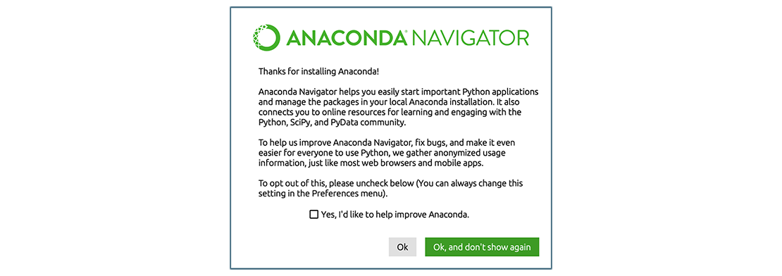 Make your choice and click “Ok,
and don’t show again” button.
 - Find the “Notebook” tab and click on the “Launch” button:
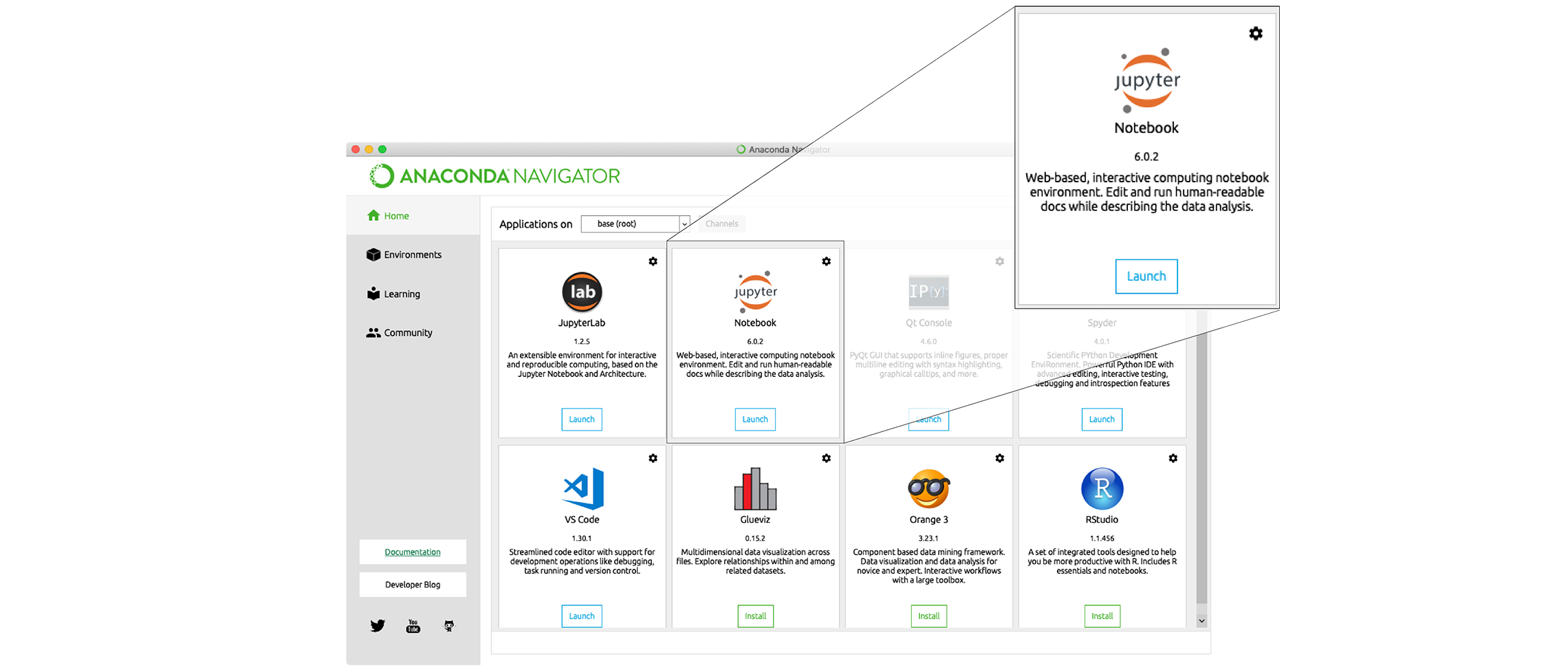 Anaconda will open a new
browser window or tab with a Notebook Dashboard showing you the contents
of your Home (or User) folder.
 - Navigate to the
datadirectory by clicking on the directory names leading to it:Desktop,swc-python, thendata: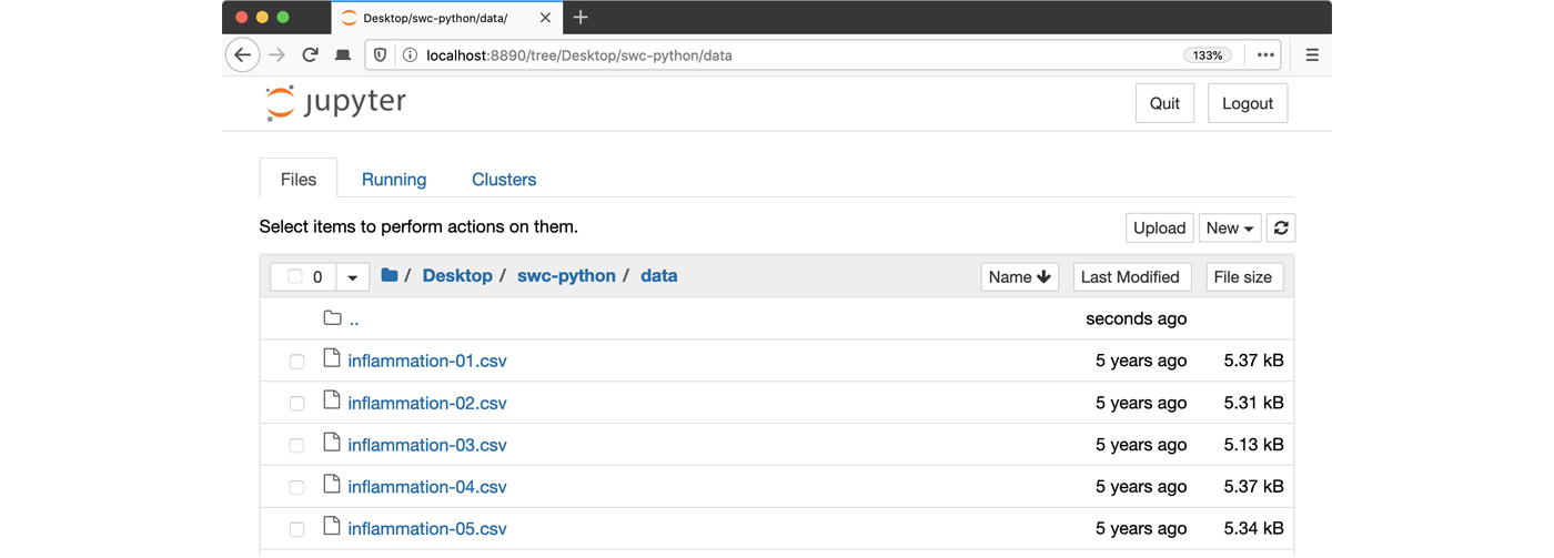
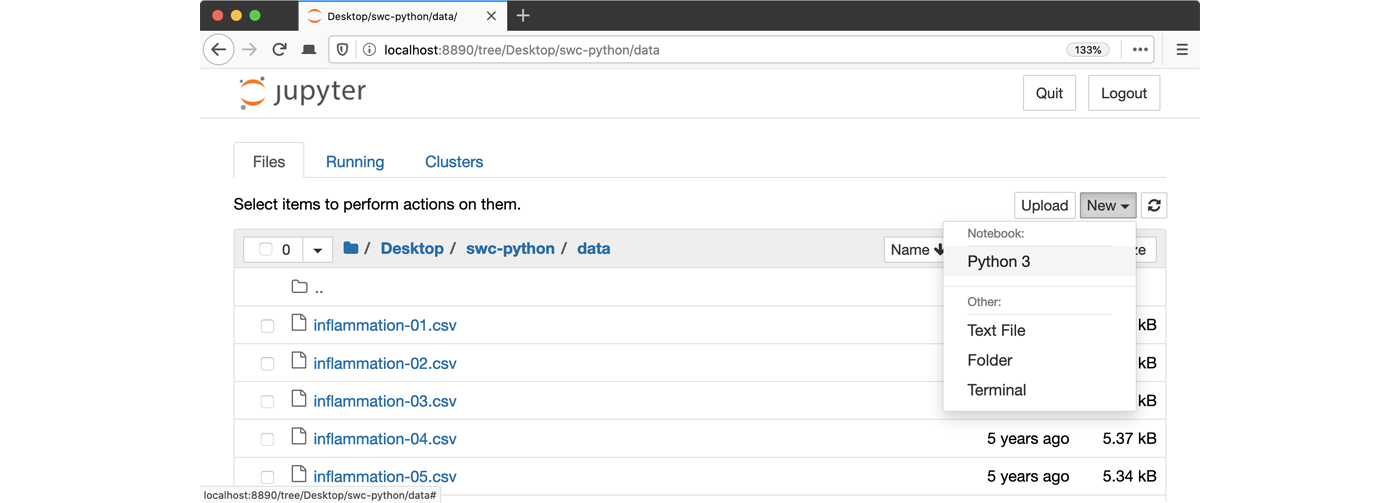
- Launch the notebook by clicking on the “New” button and then
selecting “Python 3”:
1. Navigate to the data directory:
If you’re using a Unix shell application, such as Terminal app in macOS, Console or Terminal in Linux, or Git Bash on Windows, execute the following command:
On Windows, you can use its native Command Prompt program. The
easiest way to start it up is pressing Windows Logo
Key+R, entering cmd, and hitting
Return. In the Command Prompt, use the following command to
navigate to the data folder:
cd /D %userprofile%\Desktop\swc-python\data2. Start Jupyter server
python -m notebook3. Launch the notebook by clicking on the “New” button on the right
and selecting “Python 3” from the drop-down menu: 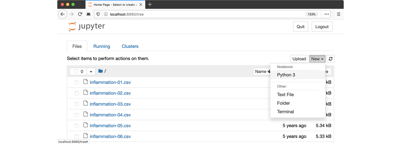
Option B: IPython interpreter
IPython is an alternative solution situated somewhere in between the plain-vanilla Python interpreter and Jupyter Notebook. It provides an interactive command-line based interpreter with various convenience features and commands. You should have IPython on your system if you installed Anaconda.
To start using IPython, execute:
ipython
Option C: plain-vanilla Python interpreter
To launch a plain-vanilla Python interpreter, execute:
pythonIf you are using Git Bash on
Windows, you have to call Python via
winpty:
winpty python