SciPy#

Overview#

NumPy provides arrays and limited additional functionality
SciPy builds on NumPy and provides additional modules:
- Linear Algebra and wrappers to LAPACK & BLAS scipy.linalg
- Numerical Integration scipy.integrate
- Interpolation scipy.interpolate
- Optimisation scipy.optimize
- Special functions scipy.special
- Signal processing scipy.signal
- Image Processing scipy.ndimage
- Fourier transforms scipy.fftpack
- Statistical functions stats
- Spatial data structures and algorithms scipy.spatial
- File I/O e.g. to read MATLAB files scipy.io

Useful links#

Note: no PDE solvers (though other packages exist)
Documentation:
- https://docs.scipy.org/doc/scipy/reference/index.html
- http://scipy-cookbook.readthedocs.org

Linear algebra: `sicpy.linalg`#

Wider set of linear algebra operations than in Numpy
- various decompositions (eigen, singular value)
- matrix exponentials, trigonometric functions
- particular matrix equations and special matrics
- low-level LAPACK and BLAS routines
Routines also for sparse matrices
- storage formats
- iterative algorithms

Example: Matrix inverse#

Consider:

\[\begin{split} A = \left[ \begin{array} {rrr} 1 & 3 & 5 \\ 2 & 5 & 1 \\ 2 & 3 & 8 \\ \end{array} \right] \end{split}\]

The inverse of \(A\) is

\[\begin{split} A^{-1} = \frac{1}{25} \left[ \begin{array} {rrr} -37 & 9 & 22\\ 14 & 2 & -9 \\ 4 & -3 & 1\\ \end{array} \right] \approx \left[ \begin{array} {rrr} -1.48 & 0.36 & 0.88\\ -0.56 & 0.08 & -0.36 \\ 0.16 & -0.12 & 0.04\\ \end{array} \right] \end{split}\]

which may be confirmed by checking \(A A^{-1} = I\) where \(I\) is the identity.

See this solution step by step!

(a) Find inverse of matrix A (as defined above).#

from scipy import linalg
import numpy as np

# Define the matrix using numpy
A = np.array([[1, 3, 5], [2, 5, 1], [2, 3, 8]])

# Find inverse using scipy.linalg.inv()
Ainv = linalg.inv(A)
print(Ainv)

[[-1.48  0.36  0.88]
 [ 0.56  0.08 -0.36]
 [ 0.16 -0.12  0.04]]

(b) Check the result by inverting the result, which should return the original matrix \(A\)#

Tip: you combine numpy.rint() to round to the nearest integer and numpy.astype(int) to transform the result into a integer matrix.

print(np.rint(linalg.inv(Ainv)).astype(int))

[[1 3 5]
 [2 5 1]
 [2 3 8]]

(c) Check the result by multiplying out \(A A^{-1}\) , which should give identity matrix \(I\)#

Were the identity matrix is:

\[\begin{split} I = \left[ \begin{array} {rrr} 1 & 0 & 0 \\ 0 & 1 & 0 \\ 0 & 0 & 1 \\ \end{array} \right] \end{split}\]

Tip: you combine numpy.rint() to round to the nearest integer and .astype(int) to transform the result into a integer matrix.

print(np.rint(A.dot(Ainv)).astype(int))

[[1 0 0]
 [0 1 0]
 [0 0 1]]

Example: Linear equation#

scipy.linalg.solve() solves the linear equation set a @ x == b for the unknown x for square a matrix.

Knowing that \(A A^{-1} = I\), find the inverse \(A^{-1}\) using the linear equation approach.

Tip: you can create an identity matrix using numpy.identity()

# define I:
I = np. identity(3, dtype=int)
print(I)

[[1 0 0]
 [0 1 0]
 [0 0 1]]

# Solving the linear equation
print(linalg.solve(A, I))

[[-1.48  0.36  0.88]
 [ 0.56  0.08 -0.36]
 [ 0.16 -0.12  0.04]]

Integration: `scipy.integrate`#

Routines for numerical integration – single, double and triple integrals
Can solve Ordinary Differential Equations (ODEs) with initial conditions

For example, we can use scipy.integrate.dblquad to determine the result of a double integral like:

\[ \int _{a} ^{b}\ \int _{g(x)} ^{h(x)} f(x,y) \, dx \ dy \]

by calling: dblquad(func, a, b, gfun, hfun), where gfun and hfun can be digits or functions.

Example : Double integral - digit boundary#

Calculate the double integral

\[ \int_0^{\pi/2} dx \int_0^1 dy \quad f(x,y) = \int_0^{\pi/2} \int_0^1 f(x,y) \ dy \ dx \]

where \(f(x,y) = y \sin(x)\). The answer should be 1/2.

# numerically integrate using dblquad()
from scipy.integrate import dblquad

# define the integrand >> arguments order is important!
def func(y, x):
    return y * np.sin(x)

# note that the result has two values: "The resultant integral" and "An estimate of the error"
print(dblquad(func, 0, np.pi/2, 0, 1))

(0.49999999999999994, 5.551115123125782e-15)

Sometimes is useful to use the inline function definition using lambda, see the same example:

# lambda arguments : expression
inline_func = lambda y, x: y * np.sin(x)
print(dblquad(inline_func, 0, np.pi/2, 0, 1))

# or in one line:
print(dblquad(lambda y, x: y * np.sin(x), 0, np.pi/2, 0, 1))

(0.49999999999999994, 5.551115123125782e-15)
(0.49999999999999994, 5.551115123125782e-15)

Example: Double integral - function boundary#

One way of testing this function is by calculating \(\pi\) using the double integral for the area of a circle with radius \(r\):

\[ \int _{-r} ^{r} \int _{-\sqrt(r^2-y^2)} ^{\sqrt(r^2-y^2)} 1 \, dx\, dy = \pi r^2 \]

We will solve this with scipy.integrate.dblquad()

Solution 1: simplify by considering \(r=1\)#

# define the integrand
def func(x, y):
    return 1

# define the lower boundary curve in x
def gfun(y):
    return -1*np.sqrt(1 - y*y)

# define the upper boundary curve in x
def hfun(y):
    return np.sqrt(1 - y*y)

my_pi = dblquad(func, -1, +1, gfun, hfun)
print(my_pi)

(3.1415926535897967, 2.000470900043183e-09)

Solution 2: generalise for any \(r\) value#

Tip: You will need call gfun and hfun using a lambda function, something like lambda y: gfun(y,r)

# define the integrand
def func(x, y):
    return 1

# define the lower boundary curve in x
def gfun(y, r):
    return -1*np.sqrt(r*r - y*y)

# define the upper boundary curve in x
def hfun(y, r):
    return np.sqrt(r*r - y*y)

# define the area for a given radius - using dblquad
def get_area(r):
    (area, err) = dblquad(func, -r, +r, lambda y: gfun(y,r), lambda y: hfun(y,r))
    return area

# get the pi value for a given area/radius:
def get_pi(r):
    area = get_area(r)
    pi = area / r / r
    return pi

my_pi = get_pi(10)
my_pi

3.1415926535897967

PI: Check result#

Compare the integrated pi value with the standard numpy.pi

# compare with numpy pi
diff = abs(np.pi - get_pi(4841))

# print with scientific notation
print(diff)

# suppress the scientific notation
print('{:.20f}'.format(diff))

6.661338147750939e-15
0.00000000000000666134

Ordinary Differential Equations: `sicpy.odeint`#

Solve Ordinary Differential Equations (ODEs) with initial conditions.

Example: Pendulum#

Considerer a point mass, \(m\), is attached to the end of a massless rigid rod of length \(l\). The pendulum is acted on by gravity and friction. We can describe the resulting motion of the pendulum by angle, \(\theta\), it makes with the vertical.

Assuming angle \(\theta\) always remains small, we can write a second-order differential equation to describe the motion of the mass according to Newton’s 2nd law of motion, \(m\,a = F\), in terms of \(\theta\):

\[ \ddot{\theta} + \frac{b}{m}\,\dot\theta + \frac{g}{l}\,\theta = 0 \]

where \(b\) is the friction coefficient and \(b \ll g\).

To use odeint, we rewrite the above equation as 2 first-order differential equations:

\( \dot{\theta} = \omega \)

\( \dot{\omega}= -\frac{g}{l}\,\theta - \frac{b}{m}\,\omega \)

Pendulum: Defining values#

Set up parameters and initial values.

# Parameters and initial values
g = 9.81                # gravitational constant
l = 1.0                 # length of pendulum
m = 1.0                 # mass of the ball
b = 0.2                 # friction coefficient
theta0 = np.radians(10) # initial angle
w0 = 0.0                # initial omega

# create a vector with the initial angle and initial omega
y0 = [theta0, w0]

# time interval
time_init = 0 # total number of seconds
time_end = 10 # total number of seconds
steps = 101   # number of points interval

t = np.linspace(time_init, time_end, steps)

Pendulum: Defining ODE#

Define the ODE as a function.

# define ODEs as a function
def pend(y, t, b, m, g, l):
    '''y = [theta, omega] '''
    theta, omega = y
    odes = [omega, - (g/l*theta) - (b/m*omega)]
    return odes

Pendulum: Solving ODE#

Define the ODE as a function.

Use odeint to numerically solve the ODE with initial conditions.

from scipy.integrate import odeint

# get solution. Note args are given as a tuple
solution = odeint(pend, y0, t, args=(b,m,g,l))

Pendulum: Exact solution & Plotting#

The ODE can be solved analytically. The exact solutions for \(\theta\) and \(\omega\) are:

# Exact solution for theta
def thetaExact(t, theta0, b, m, g, l):
    root = np.sqrt( np.abs( (b*b)-4*g*m*m/l ) )
    sol = theta0*np.exp(-b*t/2)*( np.cos( root*t/2 ) + (b/root)*np.sin( root*t/2) )
    return sol

# Exact solution for omega
def omegaExact(t, theta0, b, m, g, l):
    root = np.sqrt( np.abs( (b*b)-4*g*m*m/l ) )
    sol = -(b/2)*theta0*np.exp(-b*t/2)*( np.cos( root*t/2 ) + (b/root)*np.sin( root*t/2) ) + (theta0/2)*np.exp(-b*t/2)*( b*np.cos( root*t/2 ) - root*np.sin( root*t/2) )
    return sol

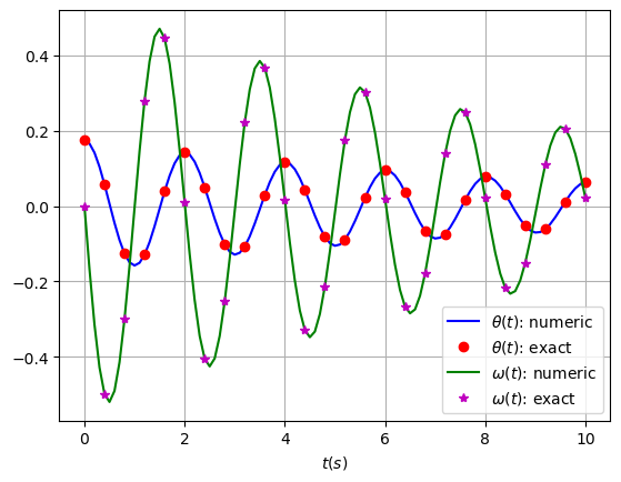
To see how good the numerical solutions for \(\theta\) and \(\omega\) are, plot the exact solutions against the numerical solutions for the appropriate range of \(t\).

You should include a legend to label the different lines/points.

You should find that the numerical solution looks quite good. Can you adjust the parameters above (re-execute all the relevant cells) to make it worse?

%matplotlib inline
import matplotlib.pyplot as plt

# plot theta
plt.plot(t, solution[:, 0], 'b', label=r'$\theta(t)$: numeric')
plt.plot(t[0::4], thetaExact(t[0::4],theta0,b,m,g,l), 'ro', label=r'$\theta(t)$: exact')

#plot omega
plt.plot(t, solution[:, 1], 'g', label=r'$\omega(t)$: numeric')
plt.plot(t[0::4], omegaExact(t[0::4],theta0,b,m,g,l), 'm*', label=r'$\omega(t)$: exact')

plt.legend(loc='best')
plt.xlabel(r'$t(s)$')
plt.grid()

Optimisation: `scipy.optimize.leastsq`#

Scipy has Several classical optimisation algorithms
- Least squares fitting
- Quasi-Newton type optimisations
- Simulated annealing
- General purpose root finding

Here, we are going to use scipy.optimize.leastsq to fit some measured data, \(\{x_i,\,y_i\}\), to a function.

Example: sin function#

Consider the following function

\[ y\,=\,A\,\sin(2\pi k x \,+\, \theta) \]

where the parameters \(A\), \(k\), and \(\theta\) are unknown.

The residual vector, that will be squared and summed by leastsq to fit the data, is:

\[ e_i\,=\, ∣∣ \, y_i \,− \,A\sin(2\pi k x_i + \theta)∣∣ \]

By defining a function to compute the residuals, \(e_i\), and, selecting appropriate starting values, leastsq can be used to find the best-fit parameters \(\hat{A}\), \(\hat{k}\), \(\hat{\theta}\).

Defining initial values#

Create a sample of “true values”, and the “measured” (noisy) data. Define the residual function and initial values.

# define the initial values
A = 10
k = 1.0 / 3e-2
theta = np.pi / 6

# define x array
points = 30
x_ini = 0
x_end = 0.06
dx = x_end/points
x = np.arange(x_ini, x_end, dx)

# parameters vector:
p = [A, k, theta]

# gessing values of the parameter vector
p0 = [8, 1 / 2.3e-2, np.pi / 3]

Function definitions#

For easy evaluation of the model function parameters y=[A, K, theta], we define two functions:

# def main function
def func(x, p):
    '''p = [A, k, theta]'''
    return p[0] * np.sin(2.0*np.pi*p[1]*x + p[2])

# Function to compute the residual
def residuals(p, measure, x):
    err = measure - func(x, p)
    return err

Experimental data#

Create an experimental data by calculating the exact solution, and then, adding a noise to it.

# define noise measured data >> tip: use random number to add noise
y_noise = func(x, p) + 2.0*np.random.randn(len(x))

Parameter estimation#

Do least squares fitting and print the parameter estimation

# least squares fitting
from scipy.optimize import leastsq

fitting = leastsq(residuals, p0, args=(y_noise, x))

# Print estimated and exact parameters
print("Estimated: ",fitting[0])
print("Exact: ",np.array(p))

Estimated:  [ 2.89311314 57.18583151 -0.54842425]
Exact:  [10.         33.33333333  0.52359878]

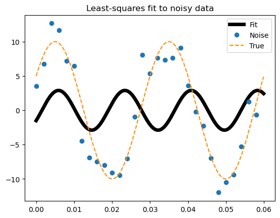
Looking the results#

# New x-vector to better plotting
x2 = np.arange(x_ini, x_end, x_end/1000)

plt.plot(x2, func(x2, fitting[0]), lw=5, c='k', label ='Fit')
plt.plot(x, y_noise, 'o', label ='Noise')
plt.plot(x2, func(x2, p), '--', color="darkorange", label ='True')

plt.title('Least-squares fit to noisy data')
plt.legend()
plt.show()

Summary#

As we have seen, SciPy has a wide range of useful functionality for scientific computing.
In case it does not have what you need, there are other packages with specialised functionality.

Other packages#

Pandas: Offers R-like statistical analysis of numerical tables and time series
SymPy: Python library for symbolic computing
scikit-image: Advanced image processing
scikit-learn: Package for machine learning
Sage: Open source replacement for Mathematica / Maple / Matlab (built using Python)

SWD5: Scientific Python

SciPy

Contents

SciPy#

Overview#

Useful links#

Linear algebra: `sicpy.linalg`#

Example: Matrix inverse#

(a) Find inverse of matrix A (as defined above).#

(b) Check the result by inverting the result, which should return the original matrix \(A\)#

(c) Check the result by multiplying out \(A A^{-1}\) , which should give identity matrix \(I\)#

Example: Linear equation#

Integration: `scipy.integrate`#

Example : Double integral - digit boundary#

Example: Double integral - function boundary#

Solution 1: simplify by considering \(r=1\)#

Solution 2: generalise for any \(r\) value#

PI: Check result#

Ordinary Differential Equations: `sicpy.odeint`#

Example: Pendulum#

Pendulum: Defining values#

Pendulum: Defining ODE#

Pendulum: Solving ODE#

Pendulum: Exact solution & Plotting#

Optimisation: `scipy.optimize.leastsq`#

Example: sin function#

Defining initial values#

Function definitions#

Experimental data#

Parameter estimation#

Looking the results#

Summary#

Other packages#

SWD5: Scientific Python

SciPy

Contents

SciPy#

Overview#

Useful links#

Linear algebra: sicpy.linalg#

Example: Matrix inverse#

(a) Find inverse of matrix A (as defined above).#

(b) Check the result by inverting the result, which should return the original matrix \(A\)#

(c) Check the result by multiplying out \(A A^{-1}\) , which should give identity matrix \(I\)#

Example: Linear equation#

Integration: scipy.integrate#

Example : Double integral - digit boundary#

Example: Double integral - function boundary#

Solution 1: simplify by considering \(r=1\)#

Solution 2: generalise for any \(r\) value#

PI: Check result#

Ordinary Differential Equations: sicpy.odeint#

Example: Pendulum#

Pendulum: Defining values#

Pendulum: Defining ODE#

Pendulum: Solving ODE#

Pendulum: Exact solution & Plotting#

Optimisation: scipy.optimize.leastsq#

Example: sin function#

Defining initial values#

Function definitions#

Experimental data#

Parameter estimation#

Looking the results#

Summary#

Other packages#

Linear algebra: `sicpy.linalg`#

Integration: `scipy.integrate`#

Ordinary Differential Equations: `sicpy.odeint`#

Optimisation: `scipy.optimize.leastsq`#